
Author: Sebastian Wagner, Automotive Simulation Center Stuttgart e.V.
In our previous blog-post we presented the results from strong scalability test only performed with Nektar++. As a next step, the code performance of Nektar++ in contrast to the commercial simulation software Fluent was investigated. The big difference are the numerical methods. Nektar++ uses a spectral/hp element method, in Fluent (DES) the Finite Volume method is implemented. In Nektar++ the polynomial expansion factors were 3 and 2 for velocity and pressure.
| Parameter | Nektar++ | Fluent |
| Reynoldsnumber | 100 | 6.3×10⁶ |
| Δt | 10-5 | 10-4 |
| Timesteps | 5000 | 500 |
| Physical time | 0.05s | 0.05s |
Table 1 summarizes the test conditions used in all calculations, presented in this blog. They were started at a physical time of 0,11s and end up at 0,16s. The different timestep sizes lead to an adaptation of their number (Table 1, line 4). As explained in [1], there is almost no noticeable difference between the computation times for both Reynolds numbers. In Figure 1 illustrates the two solvers Real time graphs. On the Y-axis the time is plotted, on the X-axis the number of cores (MPI Ranks).
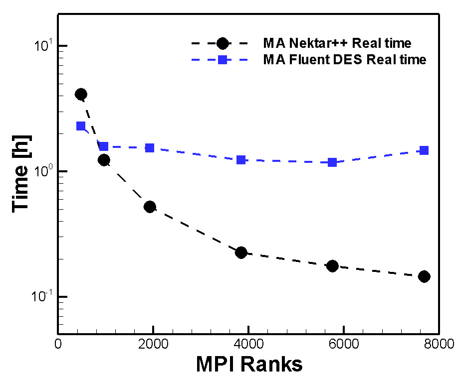
The shape of Nektar++s graph demonstrates a continuously decreasing Real time until 7860 cores. It is characterised by a strong gradient until 3840 cores and flatters off afterwards. In marked contrast to Nektar++, Fluent's Real time nearly keeps constant. Only for minimum number of cores (480) Its maximum Real time is located below Nektar++ ones. From 480 to 960 cores it's maximum Real time jump (2,3h to 1,6h) takes place. Until 5760 cores the graph shows a flat Real time decreasing. For 7860 cores it rises up to 1,46 h. The strong curves spreading begins after the point of intersection (≈900 cores). This point indicates the much better Real time values of Nektar++ compared to Fluent (DES). Reason to that is the much better scaling in contrast to Fluent (Figure 2a). The black line clearly shows its super linear scaling. The curve increases more strongly than the ideal curve up to a Speedup Value of approximately 23 (3840 cores). Further on the curve is flatten off but keeps still growing. The corresponding code Efficiency in Figure 2b increases till its optimum at 3840 cores. These two courses indicate that the ideal core number is 3840 cores.
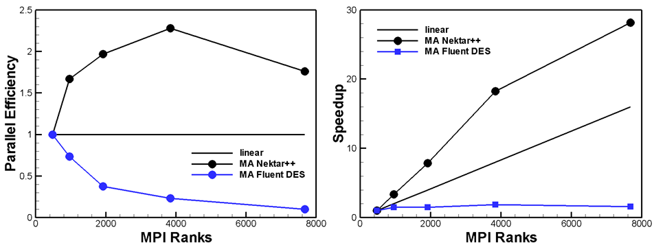
Figure 2 also reflects Fluents bad Real time reduction shown in Figure 1. Speedup values keep very low for all MPI Ranks. The maximum is reached for 3840 cores (≈1.86). Having a view on the parallel Efficiency (PE) (Figure 2b), Fluents curves decreases immediately by increasing core numbers. The blue line has its worst PE (≈ 0.15) when using 7680 cores. The facts in Figure 2 clearly show Nektar++s much better scaling behaviour. Same Message is obtained for PE and tells that Fluent is not well suited when running a simulation with high MPI Ranks.
2. Influence of a non-implicit partitioning
In this section the influence of non-implicit partitioning on the Real time is discussed. Same test conditions are used as for scalability test. With an implicit partitioning, the Real time of a calculation includes the partitioning of the computational domain into subdomains. That's why the user has to run only one job. For reducing the Real time it is possible to do a separately partitioning as a single job. Therefore, two jobs have to be run. First, the partitioning which divides the simulation domain into "n" subdomains (job run with n cores). Afterwards, this file is read during solver running.
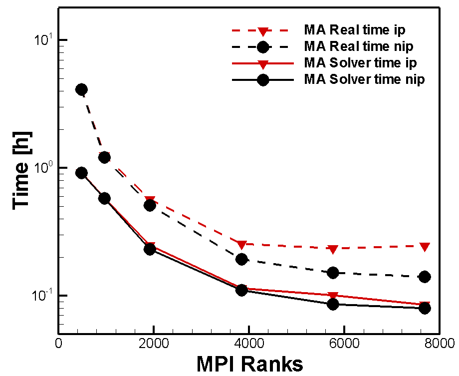
Figure 3 shows the Real- and Solver time curves for both scenarios. It illustrates that a non-implicit partitioning (nip) has no effect on the Solver time. This means partitioning time is not involved but topped on. For core numbers less than 960, partitioning has not a big influence on the Real time (curves lie on top of each other). In contrast to that course, higher core numbers (n>4000 cores) leads to drifting apart Real time curves. For implicit partitioning it keeps nearly constant, even grows up a little at 7680 cores. In the other case it continuously decreases. Due to this fact a total time and cost saving of ≈ 37.5% (5760 cores) respectively ≈ 40% (7680 cores) can be realised. Therefore, the reason is an increasing communication effort between cores when using an implicit partitioning.
3. Output files reducing with Hdf5-format
The usual output format of Nektar++ is the Xml based format. With running more complex simulations, the number of files and the data volume continuously grows up. That's why a new file format was investigated - the Hdf5-format. All calculations were run with the minimum number of required files, listed up in Table 2. Initially one can say that the initial files (without partitioning) have the same number in all calculations and are independent from the model size. The required files for initial conditions, calculated with 3840 cores, result in 3841 files.
| Name | No. of files |
| Initial conditions | 3841 |
| Boundary conditions | 12 |
| HPC Setup file | 1 |
| Nektar++ Setup-file (*.xml) | 1 |
| (mesh-file) | (1) |
| Total no. (without partitioning) | 3855 (3856) |
| Partitioning files | 3840/5760/7680 |
Every boundary (inlet, bottom, top, 2 sides) needs a data file for the three velocity components (u,v,w) which leads to 12 *.fld files. The HPC Setup-file is used to start a batch job at HLRS. It initiates the conditions- and mesh-file reading and is also used for core number definition. The Nektar++ Setup-file contains the test conditions and further on the allocation of boundary condition files to the corresponding surface. It's possible to define the mesh parameter within this file. That's why a separate mesh-file is not absolutely essential. The basic number of files depends on running a non or implicit partitioning and which MPI Rank is used for calculating the initial conditions. Using n cores means n more files through partitioning (Table 2, last row). The big difference between the file formats gets clear by comparing the number of files after calculation. With Xml-format more than ten thousand are generated- with Hdf5-format three for each MPI Rank (Table 3).
| Number of files | |||
| MPI ranks | 3840 | 5760 | 7680 |
| Xml-format | 11523 | 17283 | 23043 |
| Hdf5-format | 3 | 3 | 3 |
| Number of files | |||
| MPI ranks | 3840 | 5760 | 7680 |
| Xml-format | 3841 | 5761 | 7681 |
| Hdf5-format | 1 | 1 | 1 |
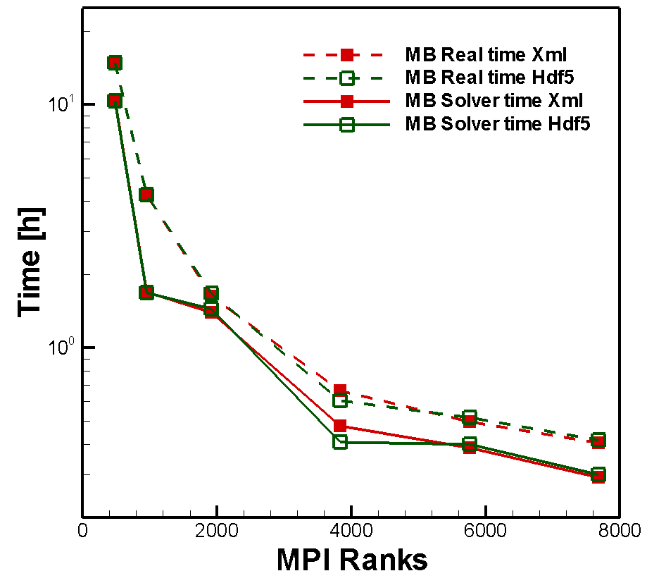
One reason are so called checkpoints which can be dumped from the user. They can be output if necessary and represent an intermediate result of the calculation. Table 4 shows the number of generated files with two defined intermediate outputs, respectively Table 5 calculations with only one generated file at the end of the calculation. In Xml-format, checkpoints are directories which includes (ncores+1) files. In contrast to that, Hdf5-format creates these checkpoints as usual data files (*.chk, 1 file). In the second point of view, the Real- and Solver time between the Xml and Hdf5-format were investigated. The line graph clearly shows the nearly identical course of the various curves. This fact indicates that the time difference between the two formats is limited to a minimum.
Reference
[2] C.D. Cantwell, et al., Nektar++: An open-source spectral/ element framework, Computer Physics Communications, 192 (2015) 205-219.