Aothors: Martin Vymazal, David Moxey, Chris Cantwell, Robert M. Kirby and Spencer Sherwin

High-order methods, combined with unstructured grids, are now becoming increasingly popular in application areas such as computational fluid dynamics. They simultaneously provide geometric flexibility and high-fidelity of flow solutions, whilst being able to utilise modern computing hardware more effectively than traditional low-order methods. These properties make high-order methods particularly attractive in various application areas such as large-eddy simulations over complex industrial geometries, which can be used to gain detailed insight into flow physics.

1. Galerkin methods in Nektar++

Nektar++ employs such high-order space discretizations inside a time-splitting scheme for incompressible Navier-Stokes equations, which repeatedly solves four scalar elliptic equations for pressure and velocity components respectively. The computation of the pressure field is the most expensive, since it is determined as a solution to a (frequently ill-conditioned) scalar Poisson equation.

Several Galerkin-type methods are available for this task, each of them have specific advantages and drawbacks [1]. The high-order continuous Galerkin (CG) method is the oldest. Compared to its discontinuous counterparts, it involves a smaller number of unknowns (as shown in figure 1), especially in a low-order setting. Discontinuous Galerkin (DG) methods [2], on the other hand, duplicate discrete variables on element boundaries, thus decoupling mesh elements and requiring at most pairwise communication between them. This is at the expense of larger linear system and more time spent in the linear solver. 

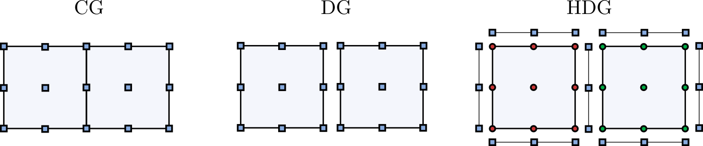
Hybrid discontinuous Galerkin (HDG) methods [3] almost recover the memory efficiency of continuous methods by introducing an additional (hybrid) variable on the mesh skeleton. The hybrid degrees of freedom determine the rank of the global system matrix and HDG therefore produces a statically condensed system that is similar in size to the CG case. The computation of the unknown variable in HDG methods consists of two stages. In the first step, a global system involving the hybrid variable is solved. Once its values are computed, the actual unknown defined independently in each element can be recovered from the hybrid values given on element trace. 

We are particularly interested in the approximation of Dirichlet boundary conditions for CG problem in weak fashion, because previous work [4] has shown that this approach has the potential of improving the stability of simulations. This is due to the fact that the forcing terms on boundary (see below) allow for simultaneous convergence of the unknown in the domain interior and on boundary towards exact solution instead of directly replacing the boundary values with exact solution when the rest of the field is still relatively far from satisfying the underlying PDE. 

The starting point for the formulation of weak boundary terms is the second HDG step, also known as local solve. Interpreting the computational mesh as one large HDG 'macro-element' with a suitable choice of approximation spaces for the scalar unknown u and its flux leads to a finite element formulation of scalar sub-problems that occur in projection schemes for incompressible Navier-Stokes equations, only this time the values that are prescribed by Dirichlet boundary conditions do not need to be lifted from the system, but are enforced by additional penalty terms instead.

2. Accuracy of Helmholtz solver – strong vs. weak Dirichlet boundary conditions

We consider a simple scalar problem to verify that the boundary constraints enforced by a penalty term converge to the exact solution with the same rate as strong boundary conditions. The underlying differential equation is of the same type that is repeatedly solved inside the incompressible Navier-Stokes solver implemented in Nektar++. Figure 2 shows the value of error norm as a function of degree of polynomials representing the numerical solution on two different grids: the first is a Cartesian quadrilateral grid, while the second consists of unstructured triangles.

Figure 2 shows that up to polynomial order 11, the errors produced by strong and weak boundary conditions are identical. With additional increase of polynomial degree, the weak errors fail to further reduce which is most likely caused by rounding errors in finite precision arithmetic. Similar behaviour can be observed when strong boundary conditions are used with the difference that the roundoff limit is reached later on (approximately for p = 14).

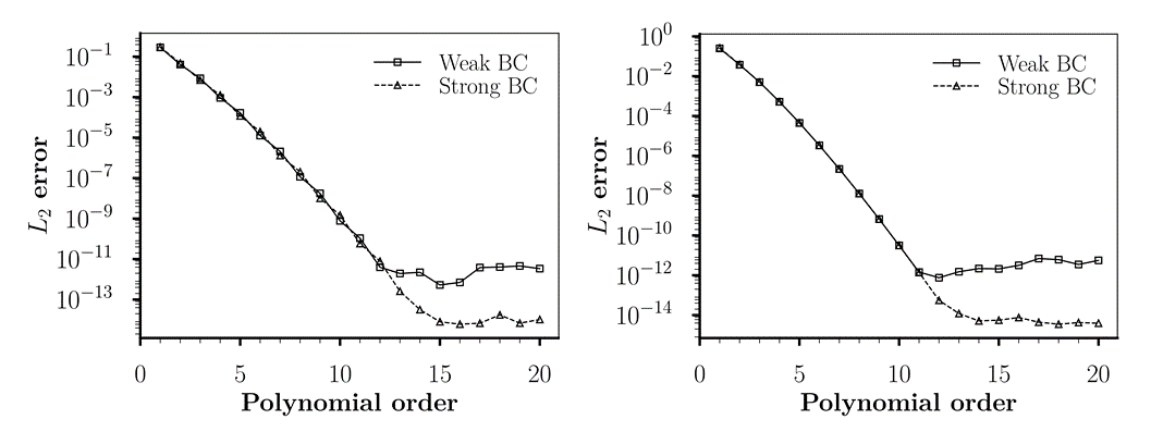
Since the boundary Dirichlet degrees of freedom are never lifted from the linear system in the weak case, the rank of the underlying global matrix is higher. This is especially important on small grids, where degrees of freedom located on domain boundary represent a significant portion of the total number of unknowns and naturally lead to systems with larger condition numbers. The observed behaviour of L2 errors (weak algorithm reaches its accuracy limit before the strong one) is therefore not entirely surprising.

3. Incompressible Navier-Stokes example

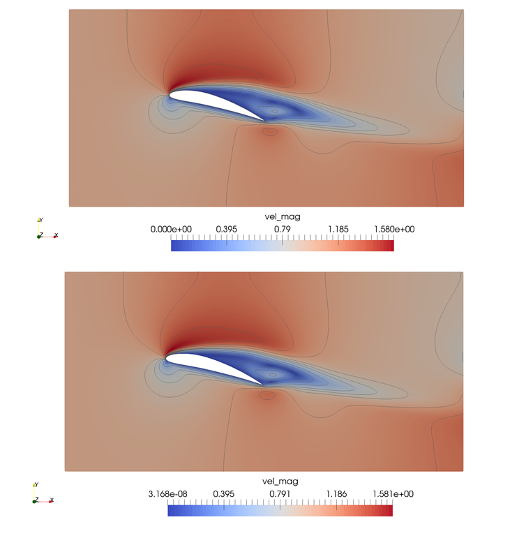
The incompressible flow past a NACA6412 airfoil was used to evaluate the performance of weak boundary conditions when computing derived quantities such as aerodynamic forces. The simulation ran for 20 000 iterations with time step ∆t = 5 x 10-3s using a velocity correction scheme implemented in Nektar++. Figure 3 shows velocity field obtained with a fifth-order method using strong (left) and weak (right) boundary conditions for both velocity components on airfoil surface. 

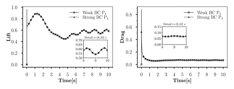
In terms of derived quantities (lift and drag), both simulations produced data that are in very good agreement (figure 4).

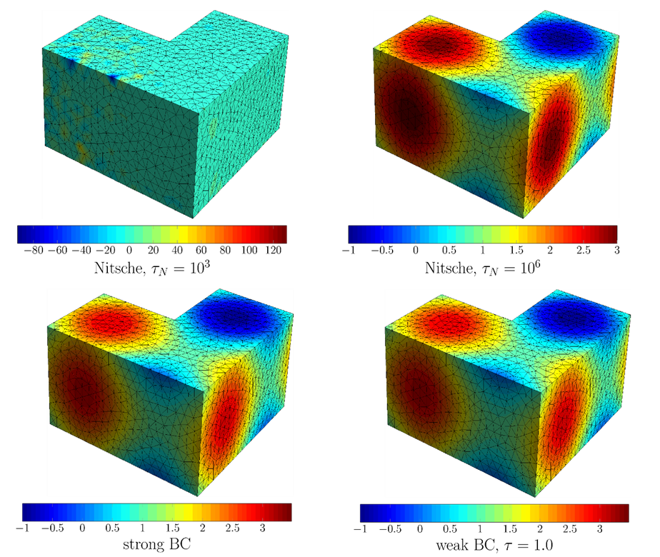
4. Nitsche’s method vs. weak boundary conditions

Nitsche’s method is the classical approach to imposition of Dirichlet boundary conditions via penalties. There is a conceptual difference between the two approaches, however. The method of Nitche augments the weak form for an elliptic problem, such as Laplace equation, by additional terms whose purpose is to guarantee that the modified problem remains well-posed. The new terms are integrated only over boundary edges (or faces in 3D), i.e. over entities of codimension 1. In addition to that, the penalty parameter employed in the formulation is a function of mesh size and hence problem dependent.

The HDG-based formulation of weak boundary conditions, on the other hand, forms additional elemental matrices in all elements that have at least one edge (face) adjacent to Dirichlet boundary. This means that we integrate over entities of codimension 0. As was the case with Nitsche, the weak form again uses a penalty parameter. This parameter, however, is not mesh-dependent (theory shows than any positive value should be satisfactory to obtain a well-posed discrete problem) and acts rather as a switch between different discretizations (continuous vs. discontinuous Galerkin) than a stability-ensuring penalty parameter. An example of the effect of the penalty parameter and comparison with strong CG algorithm is in figure 5.

References

[1] Sergey Yakovlev, David Moxey, Robert M. Kirby, and Spencer J. Sherwin. To CG or to HDG: A comparative study in 3D. Journal of Scientific Computing, 67(1):192–220, 2016.

[2] Douglas N Arnold, Franco Brezzi, Bernardo Cockburn, and L. Donatella Marini. Unified analysis of discontinuous Galerkin methods for elliptic problems. SIAM journal on numerical analysis, 39(5):1749–1779, 2002.

[3] Bernardo Cockburn, Jayadeep Gopalakrishnan, and Raytcho Lazarov. Unified Hybridization of Discontinuous Galerkin, Mixed, and Continuous Galerkin Methods for Second Order Elliptic Problems. SIAM Journal on Numerical Analysis, 47(2):1319–1365, 2009.

[4] Jan S. Hesthaven. Spectral penalty methods. Applied Numerical Mathematics 33.1-4 (2000): 23-41.