
Download material on "ExaFLOW use case: Numerical simulation of the rear wake of a sporty vehicle"
The automotive use case focuses on the simulation of an unsteady turbulent flow, which originates from the separation of the flow on the rear part of the Opel Astra GTC. This flow is characterised by the three-dimensional movement of vortical structures appearing near the rear roof spoiler. It is of interest to understand the interaction between the vortical structures and the aerodynamic coefficients in this highly sensitive region, for example the pressure coefficient cp.
Additionally to the wind tunnel testing this vehicle was aerodynamically developed by using Computational Fluid Mechanics (CFD). The Reynols number is equal Re=6.3×10⁶ using the wheel base (L=2.695m) as the characteristic length and the INLET velocity (140km/h) as reference velocity.
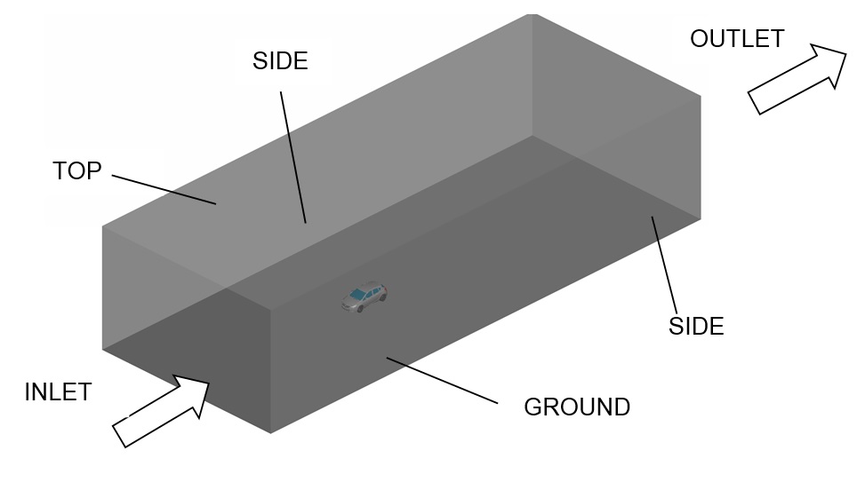
Figure 1: Computational domain of the completely vehicle model in the wind tunnel.
Numerical method
The complete simulation model consists of the entire vehicle geometry (4.468m long, 1.991m wide and 1.449 m height) and the virtual wind tunnel (51m long, 20m wide and 12m high). All boundary surfaces of the virtual wind tunnel (INLET, OUTLET, SIDE1, SIDE2, GROUND and TOP) are identified in Figure 1. At the INLET the velocity was set to a constant value of 140 kph. At the OUTLET a pressure outlet condition is applied. The symmetry condition is used on the TOP as well as on SIDE1 and SIDE2 surfaces. At the GROUND surface a moving wall condition was applied. All other surfaces of the model are set to the non-slip condition using the non-equilibrium wall function since the first cell was placed in the log-layer obtaining typical values of y+≈30.
Simulation results
The flow field around the vehicle is illustrated in Figure 2. The flow is characterized by a big stagnation point at the front part of the vehicle and a smaller one at the windshield. Low velocity values are depicted in the airflow through the engine compartment and underbody as well at the wake of the vehicle. The location of the main turbulent structures are identified by the isosurface of the total mean pressure <p>=0 bar as illustrated in Figure 3. The isosurface is colored by the Turbulent Kinetic Energy k and shows that the main structures originate from each wheel (4 Structures), each sidemirror (2 Structures) and from the rear end of the vehicle (1 Structure).
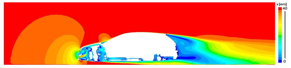
Figure 2: Simulation results (RANS) of the complete vehicle model. 2D contour of the velocity magnitude at the middle of the vehicle.
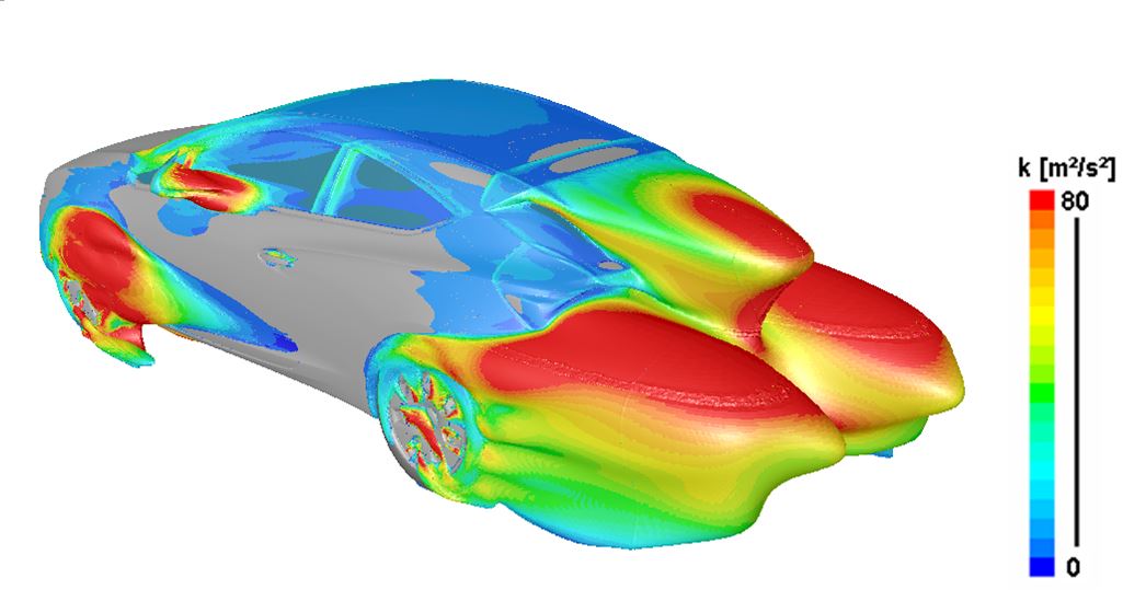
Figure 3: Simulation results of the complete vehicle model. 3D isosurface of the mean total pressure <p> = 0 bar.
CODES USED: Nektar++