Author: Nicolas Offermans, KTH Royal Institute of Technology

In our previous blog posts, we presented our progress on the implementation of h-type mesh refinement capabilities in the spectral element method (SEM) code Nek5000. For the next step, we combine these tools with appropriate error estimators and we perform adaptive mesh refinement (AMR) on some test cases. Two methods are considered for estimating the error. The first method uses selected spectral error indicators, which are based on the properties of the SEM. The second one uses dual error estimators, which are based on the computation of an adjoint problem. At the moment, only steady and two-dimensional simulations are considered. Yet, the results obtained provide a valuable experience before an application to the real-world benchmarks/test cases of the ExaFLOW project in the future. A detailed description of our latest work can be found in [1].

A posteriori error indicators can be computed based on the solution variation on a given grid. We follow a method developed by [2], where the error estimate is the sum of the truncation error and the quadrature error. These indicators estimate the local error within the domain (typically based on local velocities, gradients, vorticity, etc.) such that the sum of all the local contributions gives an estimate of the total error on the solution. The adjoint error estimators, on the other hand, estimate the error on a given functional (typically drag, lift, heat transfer, etc.) based on the global sensitivity of the target to the solution. Therefore, adjoint error estimators are used to optimally predict some quantity of interest. The derivation of such estimators for the SEM follows a method developed in [3] for the finite element method.

We demonstrate the use of AMR on the two-dimensional flow past a cylinder at a Reynolds number Re=40. At that regime, the flow is laminar and consists of a pair of steady vortices behind the cylinder. The configuration of the case and the original mesh are illustrated in Figure 1, as a function of D, the diameter of the cylinder. When using the adjoint error estimators, it is necessary to define a functional of interest, which determines the adjoint boundary conditions. We choose the drag on the cylinder, such that the boundary conditions for the adjoint problem are a non-zero velocity, oriented in the opposite direction to the bulk of the flow, on the cylinder's surface and zero velocity everywhere else.

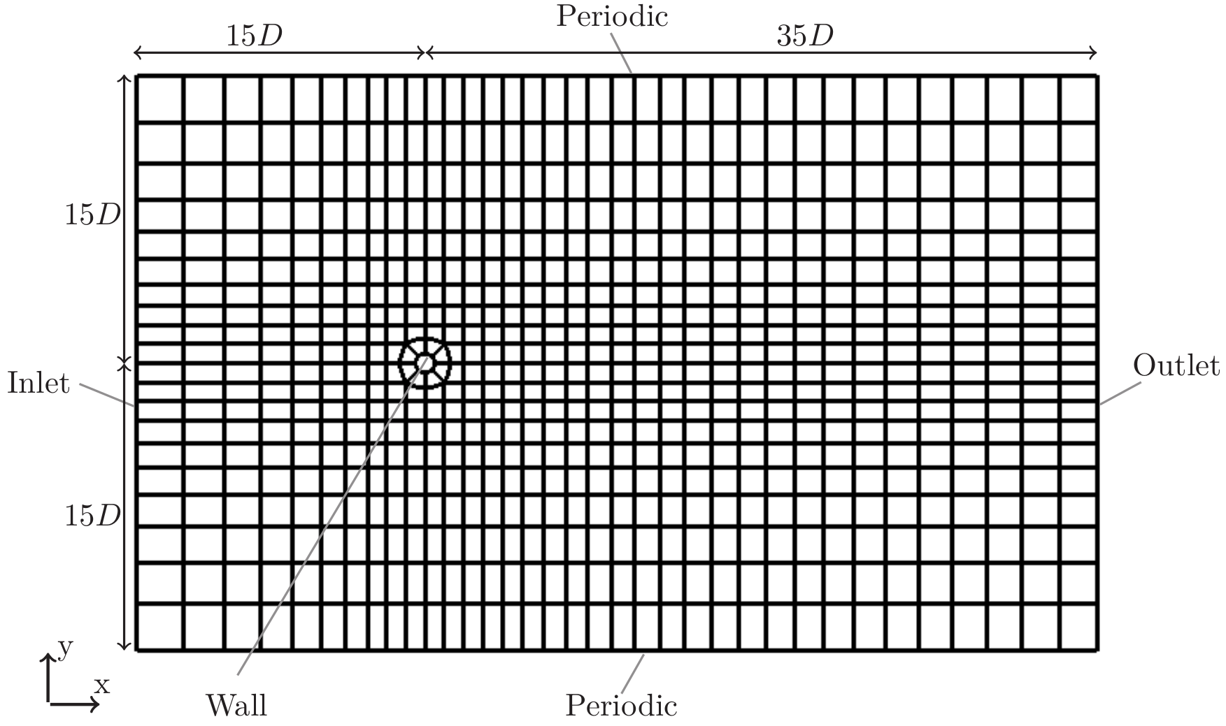
Figure 1 - Original mesh for the flow past the cylinder.

The same refinement strategy is used for both error estimators. Since we consider steady cases only, the mesh converges toward an optimal state and we do not need to perform coarsening. First, a steady solution is obtained for the direct problem and also the adjoint problem if required. Then, a local error is computed on each element depending on the chosen method. All elements that satisfy some refinement criterion are marked and refined, unless a predefined maximum level of refinement is reached. This process is repeated until some stopping criterion is satisfied. The evolution of the mesh and the convergence of the drag when using both methods for estimating the error can be analysed. An element is marked for refinement if its local error is higher than a certain fraction, chosen to be equal to 0.1 for the particular case of the cylinder, of the maximum local error over the whole mesh. The maximum refinement level is 4, i.e. an element can be refined maximum 4 times.

The evolution of the mesh on a zoom around the cylinder when spectral error indicators are used is shown in Figure 2. The same plot in the case of the adjoint error estimators is illustrated in Figure 3. In both cases, the refinement starts around the cylinder and propagates around it, with the most refined regions always being close to the cylinder's surface. With the spectral error indicators, the refinement follows the wake of the cylinder, where velocity gradients are high, and propagates more downstream. With the adjoint error estimators, refinement propagates upstream more than it does downstream. For both error estimators, the maximum level of refinement is reached after four steps of refinement (picture on the third row, left) for some of the elements. After seven steps of refinement (picture on the fourth row, right), further refinement is prevented because of the imposed maximum level of refinement and this translates into no significant decrease in the error, as will be shown shortly.

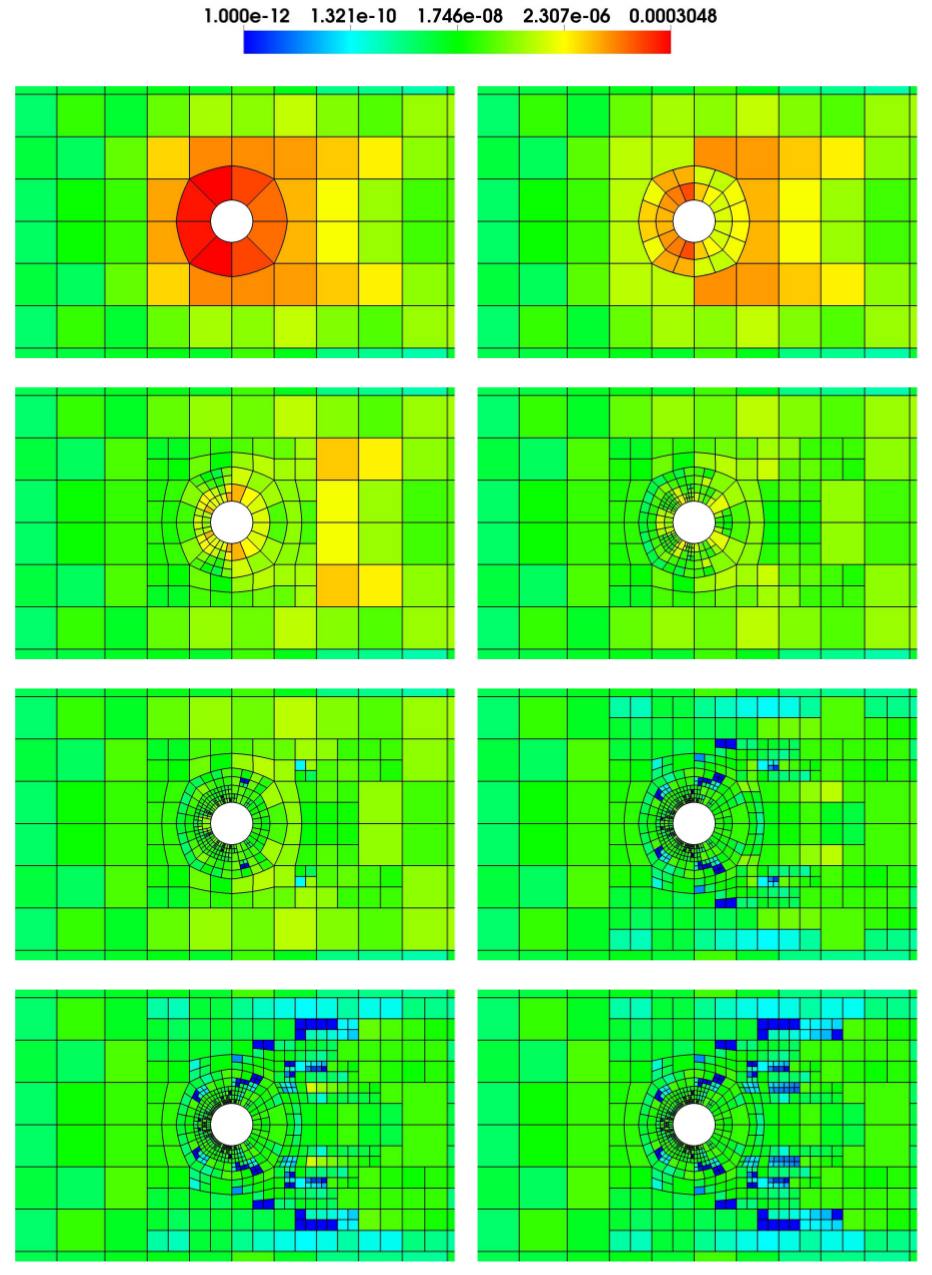
Figure 2 - Spectral error indicators as the mesh is refined around the cylinder (from left to right, from top to bottom).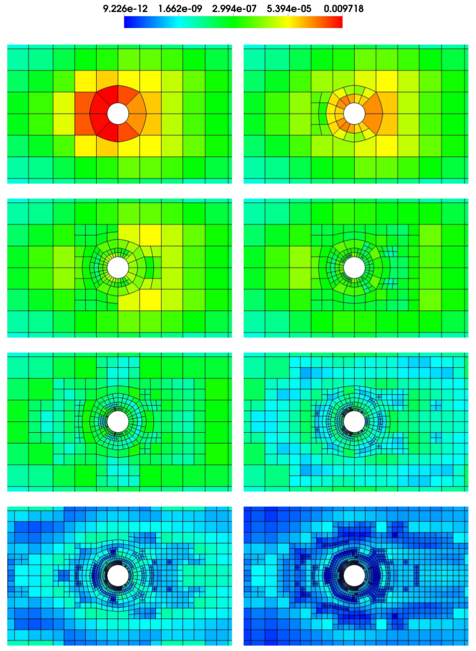

Figure 3 - Adjoint error estimators as the mesh is refined around the cylinder (from left to right, from top to bottom).

In addition, we study the convergence of the error on the drag as refinement proceeds. The reference value for the drag is computed on a conforming mesh made of 5322 elements. The error on the drag as a function of the number of elements when using AMR is shown in Figure 4.  We observe that the error on the drag converges rapidly for both methods. After about five rounds of refinement, the error on the drag stalls because the maximum refinement level has been reached for the critical elements. The use of adjoint error estimators reduces the final error on the drag by a factor 3 approximately compared to spectral error indicators.

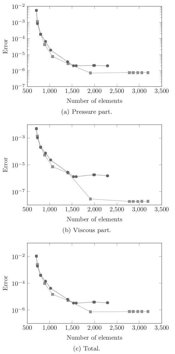
Figure 4 - Error on the drag on the cylinder when using the adjoint error estimators (square) and when using the spectral error indicators (circle).

In the future, adjoint error estimators will be extended to unsteady flows and more complex test cases will be considered. The development of time dependent estimators will ideally make use of an efficient checkpointing strategy (see [4] for example), which would ensure an efficient adjoint computation. In our study, we also observed that the presence of nonconforming elements does not modify the physics or the stability of the flow for the simple test cases considered. However, in the case of turbulent flows, noise can occur at the intersection between a fine and a coarse regions. The implementation of a proper filtering method is currently under investigation to mitigate this effect.

[1] Offermans, N. (2017). Towards adaptive mesh refinement in Nek5000 (Licentiate dissertation). Retrieved from http://urn.kb.se/resolve?urn=urn:nbn:se:kth:diva-217501

[2] Mavriplis, C. (1990) A posteriori error estimators for adaptive spectral element techniques. In Notes on Numerical Fluid Mechanics (ed. P. Wesseling), pp. 333-342.

[3] Bangerth, W. & Rannacher, R. (2002) Adaptive Finite Element Methods for Differential Equations. Birkhäuser, Basel.

[4] Schanen, M., Marin, O., Zhang, H. & Anitescu, M. (2016) Asynchronous two-level checkpointing scheme for large-scale adjoints in the spectral-element solver nek5000. Procedia Computer Science 80 (Supplement C), 1147 – 1158, international Conference on Computational Science 2016, ICCS 2016, 6-8 June 2016, San Diego, California, USA.