Author: Carlos J. Falconi Delgado, Automotive Simulation Center Stuttgart e.V.
The computational methods which fully take into account the evolution of three-dimensional turbulent behaviors such as LES and DNS require huge computation cost according to the temporal and spatial resolution of those approaches. Using a code with a good scalability behavior would enable more efficient computation in order to meet the fast turnaround times (<36 hours) required from the automotive industry. To find the optimal number of processors for massive computation, the computation time with respect to the number of cores, namely strong scalability test has been carried out.
Strong scalability test with the automotive use case
The strong scalability test has been performed by nektar++ in the HLRS facility Hazel Hen. The zero initial velocity is specified and Reynolds number is set to 1,000. The influence of Reynolds number has also been investigated with Reynolds number of 10,000. There is almost no noticeable difference between the computation times for both Reynolds numbers. In the future, the Reynolds number will be increased to reach Re=6.3×10⁶ used for DES simulation[1]. The expansion factors are used 3 and 2 for velocity and pressure, respectively. The calculation runs till 5000 iteration with time step size of 1×10⁻⁵ so that it comes up with the same physical time, 0.05s.
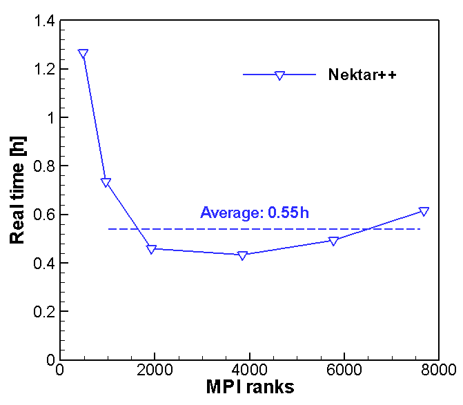
Figure 1: Comparison of real time between fluent DES and nektar++ for the physical time of 0.05s with different number of processors.
Real time comparison
The ‘real time’ represents that the waiting time for user from the job submission till the end of the job. Figure 1 shows the real time of the scalability test. As the processor number increases, the real time is decreasing till the 3840 number of cores. With more than this number of cores, the real time is increasing again. The average time of nektar++ for 960~7680 cores is 0.55h.
Solver time vs real time
There is another time for the computation namely ‘solver time’ in nektar++. This solver time represents the time required for the solver. This information is written at each output frequency specified by user and finally the sum of these times is also written as ‘Time-integration’ at the end of output file. This solver time is therefore always less than the real time. The solver time for first time step is given in Table 1 with different number of processors. The time for 1st time step is much longer than the average time per time step. The time for first time step may contain all the time for preparation of calculation such as decomposition before starting calculation. Therefore, this time is excluded for the average time evaluation.
| MPI ranks | 480 | 960 | 1920 | 3840 | 5760 | 7680 |
| 1st time step | 97s | 67s | 51s | 42s | 33s | 41s |
| Average time per time step | 0.8s | 0.4s | 0.21s | 0.11s | 0.073s | 0.066s |
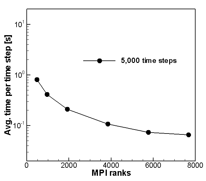
Figure 2: Average solver time per time step from three different calculations with 5,000 time steps.
Figure 2 compares the average solver time per time step with respect to the number of processors. This average solver time is evaluated by dividing the Time-integration by number of time steps without first output frequency. As depicted in Figure 2, the average solver time is decreasing as MPI rank increases. Even if the slope of decrease is being smaller, the solver time is gradually decreasing as the number of core increases. For 5000 time steps, using more than 5760 cores requires less than 1s per time step and the time for 5760 and 7680 cores are almost similar.
Initial evaluation of ExaFLOW developments
The usual output method of nektar++ is the xml-based format which writes separate files per each MPI rank. Recently, hdf5 method, a hierarchical method with a combined output file, is implemented to nektar++. This implementation has been accomplished during this project period. As an evaluation of the development in other working package, the scalability test for hdf5 has been also performed to compare the computational time from the original xml-based format.
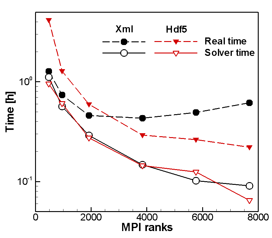
Figure 3: Total solver time and real time with respect to the number of cores. Comparison between Xml (black colored) and hdf5 (red colored) output format.
Improvement of real time
The computation times with two different output formats (xml and hdf5) in nektar++ are compared in this section. Figure 3 shows the results of strong scalability test for nektar++ with both output formats. This plot compares the total solver time and real time with increasing the number of processors. As already shown in Figure 2, the solver time using the xml format is decreasing as MPI rank increases. Hdf5 results show also similar trends of solver time against increasing number of cores. However, the real times for both methods deviate remarkably. The real time of xml format starts increasing with more than 3840 cores so that this number of cores is optimal to minimize computation time using this format. In contrary, the real time with hdf5 format is gradually declining by increasing number of processors. The new output format shows notable reduction of computation time for high MPI rank.
The computation times depicted in Figure 3 and the reduction rate (Eq. (1)) with hdf5 format are given in Table 2.
(1) Reduction rate = Abs(Hdf5 real time – Xml real time)/(Xm 1 real time) x 100
The real time of hdf5 format with highest MPI ranks is 64% smaller than that of xml format. However, hdf5 requires longer time where the number of CPUs is smaller than 1920. With smallest number of cores, the real time of hdf5 format is almost four times longer than the real time of xml format. Currently, the hdf5 format is therefore suitable for use more than 3000 processors.
| MPI ranks | 480 | 960 | 1920 | 3840 | 5760 | 7680 |
| Xml: Total solver time, h | 1.12 | 0.567 | 0.290 | 0.147 | 0.102 | 0.091 |
| Xml: Real time, h | 1.26 | 0.736 | 0.460 | 0.433 | 0.494 | 0.616 |
| Hdf5: Total solver time, h | 0.953 | 0.608 | 0.275 | 0.144 | 0.124 | 0.065 |
| Hdf5: Real time, h | 4.16 | 1.277 | 0.594 | 0.292 | 0.264 | 0.221 |
| Reduction rate of real time, % | -229 | -74 | 29 | 33 | 47 | 64 |
Reference
[1] C.J. Falconi, D. Lautenschlager, ExaFLOW use case: Numerical simulation of the rear wake of a sporty vehicle, ExaFLOW technical report, 2016, http://exaflow-project.eu/index.php/use-cases/automotive.
[2] C.D. Cantwell, et al., Nektar++: An open-source spectral/ element framework, Computer Physics Communications, 192 (2015) 205-219.