SEGL User Manual
T. Krasikova, Y. Yudin, Y. Dorozhko
27 September 2010
Contents
1 Introduction
1.1 Purpose and Scope
1.2 Terms, Definitions and Abbreviations
1.3 References
1.4 Overview
2 How to install and run the client application
3 Connecting to the server
3.1 Network settings
3.2 Network server address
4 Basic available actions
5 Programm navigation
6 Creation and editing an module
6.1 Module implementation
7 Creation and editing of experiment model
8 Start of the experiment and monitoring
Chapter 1
Introduction
This User manual document uses RUP and IEEE Standard 1016-1998, IEEE Recommended Practice for Software Design Descriptions, as a basis and it was tailored to meet the specific project needs.
1.1 Purpose and Scope
This document provides a comprehensive architectural overview of the client application, using a number of different user views to depict different aspects of the application.
Number of these views can clearly imagine the system to each interested person (stakeholder).
The document is intended for end users, as well as for persons which are responsible for the system support.
This description of the client application defines the implementation details of the system in terms of end user, but does not define the fundamental approaches and problems in the subject area. Also this document does not use the concepts of language GriCoL.
1.2 Terms, Definitions and Abbreviations
| Name | Abbreviation | Description |
| Science Experimental Grid Laboratory | SEGL | |
| Virtual Organization | VO | |
| Demilitarized Zone | DMZ | |
| Front-end | | |
| Portable Batch System | PBS | |
| Data Transfer Object | DTO | |
| Inversion of control | IOC | |
| Create, Read, Update | CRU | |
| Access Control List | ACL | |
1.3 References
| RUP | Rational Unified Process |
| IEEE-Std-1016-1998 | IEEE Recommended Practice for Software Design Descriptions |
| [SRS] | Project.SRS.doc - project requirement specification |
|
refs/GFD.147.pdf |
| http://forge.ogf.org/sf/projects/glue-wg |
| GLUE2 specification |
| refs/experimentModel.xsd | XML schema of experiment model description |
|
refs/GFD.56.pdf |
| https://forge.gridforum.org/sf/projects/jsdl-wg |
| JSDL specification |
| refs/moduleOnJsdl.xsd | XML schema of the executable module description |
|
refs/springsecurity.pdf |
| http://static.springsource.org/spring-security/site/ |
| Spring Security documentation |
1.4 Overview
The document consists of several chapters that consistently define the client application. However, not necessarily read the document strictly sequentially. For example the chapter "Start of the experiment and monitoring" defines work with input and output data of the experiment, process of starting the experiment and monitoring of it. This chapter is independent and can be read in isolation from other chapters.
Chapter "How to install and run the client application" defines the main tasks to install and start the client application.
Chapter "Connecting to the server" introduces parameters of network, that must be configured to create a new network connection from the client program to the SEGL server.
Chapters "Basic available actions" and "Programm navigation" describes location of base control elements of the client application. In these chapters information about menu, buttons, control elements and navigation in the program can be found.
Chapters "Creation and editing an module" and "Creation and editing of experiment model" talk about process of creating executable modules and experiment models. These chapters can be useful for users, who want to create new model of the experiment instead of using existent models to start new experiments.
Chapter "Start of the experiment and monitoring" describes in details how new experiment can be started. There is detail description of process of configuring new experiment, setting input data. After starting, experiment can be monitored. And the monitoring of the runned experiment is also described here. After finishing, user can analyze structure of output data tree and get output data.
Chapter 2
How to install and run the client application
The client application, then Experiment Designer, should be installed and started using the WebStart system. To start the Experiment Designer on the user's computer must be running Sun JRE 6 with WebStart. If you have not already installed Sun JRE 6, you can download the software here:
http://java.com/ru/download/index.jsp
To install and work with the Experiment Designer network connection to the SEGL server is required.
To install the Experiment Designer it is necessary in the Internet browser (e.g. Internet Explorer or FireFox) to follow the special link. This link and login / password you can get from your system SEGL administrator. Link looks like this: https://asgard.hlrs.de:1098/seglclient/webstart/client.jnlp
When you follow this link the browser initiates the WebStart system. The WebStart system will get Experiment Designer application from the SEGL server, will install it on your computer and will run. During installation you will be able to confirm your confidence to the SEGL server through its certificate and to the Experiment Designer, whose installation files are signed with a server certificate.
If you see on your screen following items are prompted to enter your login and password.
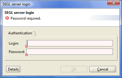
Figure 2.1: Login window.
It means that Experiment Designer has been successfully installed and started on your computer. Each time when you start Experiment Designer, newer versions of the program will be automatically checked on the SEGL server. If the server has a newer version of the program, it will be automatically downloaded and installed.
To start the Experiment Designer, which has been previously installed on your computer using WebStart system, the user can use the various options. The user can click on the above mentioned link in the web browser. This starts the Experiment Designer. The user can also use the program icon on the desktop or Start→Programs (path in the menu depends on your operating system and is different for Windows and Linux). In some versions of Linux-like operating systems, desktop icons should be confirmed by the user during or after installation on your computer.
Chapter 3
Connecting to the server
3.1 Network settings
If you use the Internet from your computer via the Proxy-server, you may need additional configuration parameters for Java applications, so they can properly use the Proxy-server. To do this, run the Java application Control Panel. This application can be run by executing javacpl in the console.
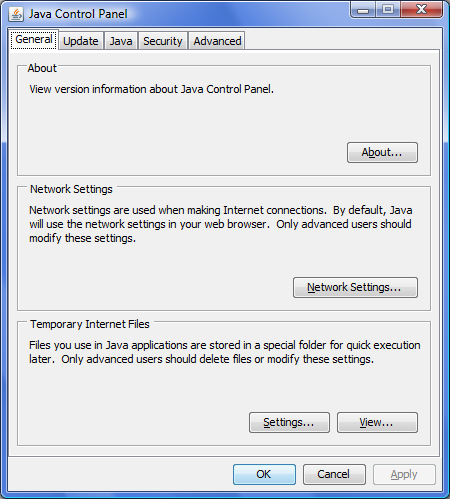
Figure 3.1: Java Control Panel window.
On the General tab, click "Network Settings" .... Then in the corresponding dialog box, make the setting to work with the Proxy-server.
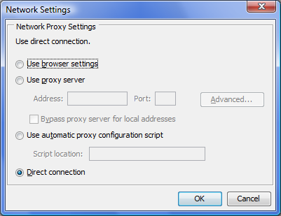
Figure 3.2: Network Settings window.
But usually when you install Java on your computer, these settings do not require changes, and the system works correctly with the network settings, performed in default mode.
3.2 Network server address
After running the application in the authentication dialog, the user can specify the desired network address of the server, which then connection is established. To do this, click Details, and enter the desired address.
ATTENTION! The server address is specified with the protocol (https) and server port (1098)
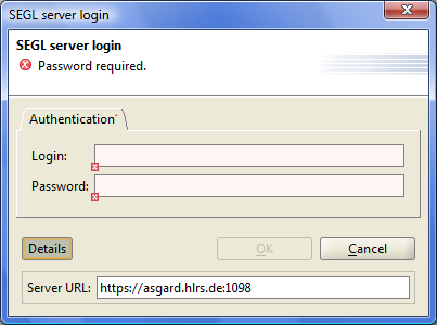
Figure 3.3: SEGL login window.
In the case of a successful connection to the server and user authentication, you will see the following window:
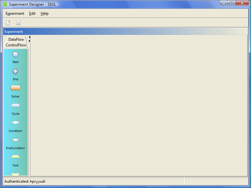
Figure 3.4: SEGL main window.
In the lower left corner of the window the user name is shown (Authenticated:), who is currently authenticated to the system. For information about the version of Experiment Designer, the server version of SEGL and address of the server, select the main menu Help→About.
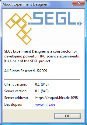
Figure 3.5: About SEGL window.
Chapter 4
Basic available actions
Item "Experiment" in the main menu of the program contains all the basic actions available to the user.
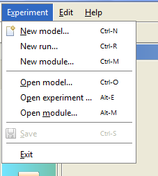
Figure 4.1: Main menu.
Let us consider the appointment of these actions:
- New model - creation of a new model of the experiment. Allows you to describe a new model of computing experiment with GriCoL language. This model will be stored on the SEGL system server. Based on this model you can run experiments with the real data (see "New module").
- New run - allows you to create a new experiment by selecting the previously created model. Created experiment will be runned on the HPC resources. This will use the input data provided by the user at the time of start of the experiment.
- New module - allows to describe the computing module, which can then be used to create models of experiments. Each computer module should have a set of implementations that are intended to run the module on different computing resources. Minimum number of implementations equal to unity.
- Open model - allows you to open one of the models identified in the system for viewing and editing.
- Open experiment - allows you to open for monitoring the running earlier (see "New run") experiment. At the time of execution of the action this experiment may be in the process of running or to be completed.
- Open module - allows you to open one of the modules defined in the system for viewing and editing.
Chapter 5
Programm navigation
In the program can be simultaneously open for editing or viewing the set of experiments, experiment models and modules. You may switch between windows of this objects by using the top tab bar.
Some objects in the system, such as model experiments, can have multiple editing windows. For example, the model of the experiment can be opened in the main window that displays ControlFlow of this model and also: the window which displays a set of Data spaces of this model and the window for editing the Data Flow models of different blocks of the experiment. Switching between these nested windows is performed by using the bottom tabs.
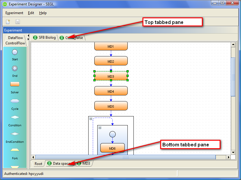
Figure 5.1: SEGL navigation tabs.
To save any changes, use the "Save" button in the main toolbar, the keyboard shortcut Ctrl+S, or internal main menu Experiment→Save. This will save all the changes of the current active window (the active tab at the top of the tab bar).
ATTENTION! When you save the experiment models and modules, all changes will be saved to the SEGL server system. This means that the stored model or modules become available for editing and usage for other users who have proper rights in the system.
Chapter 6
Creation and editing an module
Creation of a module is performed using the main menu item Experiment→New module. Before describing the generated module, the user must specify a unique name to identify the module. The name of any module of the system can be changed by the user, in case that the new name of the module will also be unique.
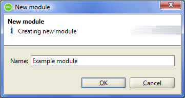
Figure 6.1: Set name of new module.
After specifying the new name of the module, the program will open a tab with the given name and a window for editing an module. Similarly, you can open for editing an existing module in the system, using the main menu of the program Experiment→Open module.
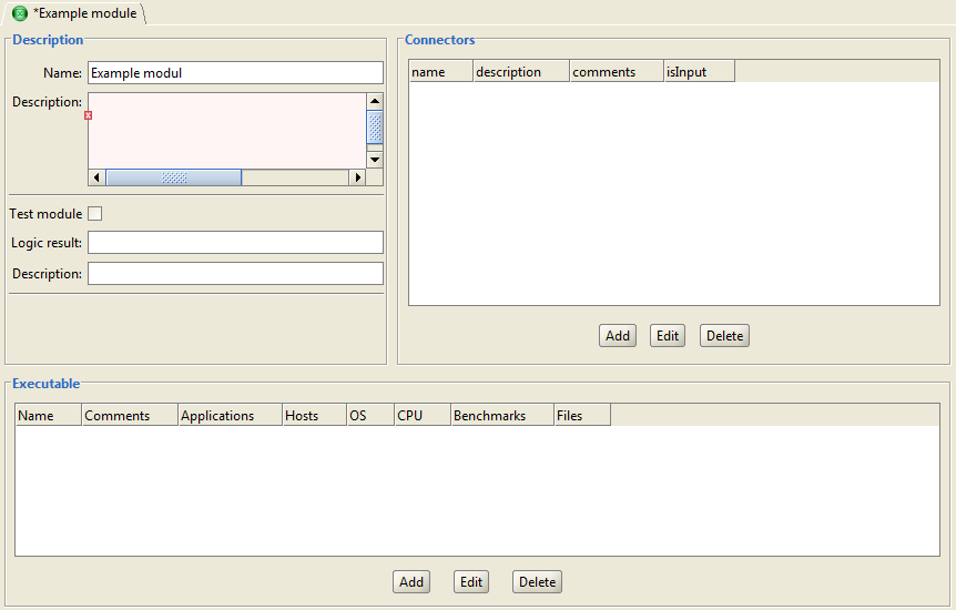
Figure 6.2: Create module window.
The editing module window consists of three panels: Description, Connectors, Executable.
Fields Name and Description determine the short and full description of the module.
The executable module can be of two types - normal module that implements a computational problem and the test module, which on the results of a computational problem returns a boolean "true" or "false" values. In addition to the boolean test module can return the usual results of the computational problem in the form of files.
Test modules are used for Condition blocks to determine the further branching of the implementation of the experiment and in cycles, to determine the out conditions of the cycle.
Check box "Test module" determines - whether the module test or normal computing module.
Field "Logic result" determines the type of test module. Currently allowed to use in this field only one value: FILE_PRESENT. This means that the module on the results of the computational problem fixes a boolean value with the file. The file name is specified in the field Description. If, after completion of the module system detects a file in the working directory with the given name, it is considered that the test module returns a boolean "true". If there is no such file in the working folder, this means that the test module returned a boolean "false" value.
Panel Connectors allows to create, edit and delete the module connectors.
Connector is a point of connection to the module, the point through which the module as an executable program receives input and gives output files. Connectors defined in the module are used during the execution of the experiment to the transfer of input files to the executable program and to save the output files of the program. Connector of the module also have a graphic image when working with modules at the DataFlow.
Connectors are divided into input and output. However, the module can not have both input and output connectors. This means that the system SEGL at the time of start the program should not give it any input files, and after the completion of the program will not save any output files. It is possible that the program will receive and store data through their own mechanisms, independent of the SEGL system.
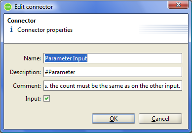
Figure 6.3: Edit Connector window.
When editing / creating the connector, you must specify its name in the "Name" field and the description in the "Comment" field. Value of description field depends on the type of connector, input or output.
Description field for the input connector is used as a special string. When the program starts to execute, the system will run a predefined shell-script. This shell-script is defined for each implementation of the module (see "Executable"). In this script, all the file names that are the input data, replaced by a special string values. Exactly the same special string value should be defined in one of the input connectors.
For example, to start the module on one of the HPC resources shell-script are used, which has the following lines:
#!/bin/bash
#
#PBS -l nodes=1,walltime=0:25:00
#PBS -e err.out
#PBS -o std.out
FITNES_NEED=12
outFitnesFile=Fitness_Best
outParameterFile=Parameter_Best
parameterFiles=( #Parameter )
fitnessFiles=( #Fitness )
parameterFiles and fitnessFiles variables determine the values of the names of input files.
This module input connectors (Parameter Input and Fitness Input) will look like this:
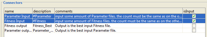
Figure 6.4: Connectors list.
When you run the module will be launched this script. Instead the values of #Parameter and #Fitness necessary file names will be substituted in a script. It is possible that instead of the value of each line will be replaced by not one, but more files using the symbol " " as a separator.
Description field for the output connector is used to determine the name or file mask. After completion of the module, the system will find the file in the working folder and save information about the file in the system. It depends on the description of the experiment at the Data flow.
Presented in this example, the connectors at the level Data flow look like this:
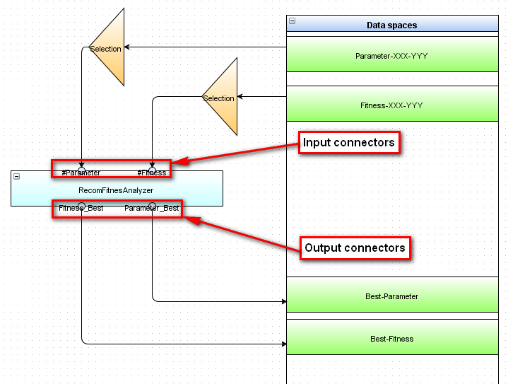
Figure 6.5: SEGL Data flow.
6.1 Module implementation
Panel "Executable" in the edit module window allows you to add, delete and edit the implementation of the executable module. Each module implementation is designed to run this module on certain HPC resource.
Fields "Name" and "Description" contain a brief and detailed description of the implementation of the module.
Applications, Hosts and Benchmarks lists can identify resource requirements, on which this module implementation will be launched.
- "Applications" - determines the necessary Software, which should be available on the HPC resource.
- "Hosts" - defines a list of resources on which this implementation can be started. If none of the resources is selected, it is considered that the implementation can be run on any available resource.
- "Benchmarks" - defines a list of indicators of resource productivity, which are important for the implementation of this module when the system selects the resource in the runtime.
In the text box "Start" shell-script must be defined, which will be launched on the HPC resource. This script should be written considering to the work with module connectors (see above).
Table "Module files" allows you to download additional files needed for the work of the implementation of the module and mark them as executable, if necessary.
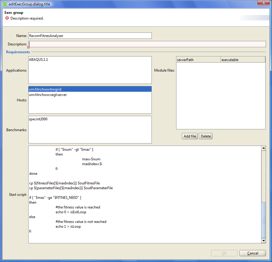
Figure 6.6: Creation of module.
Chapter 7
Creation and editing of experiment model
Creating of experiment model is performed using the main menu item Experiment→New model. Editing of an existing experiment is performed using the main menu item Experiment→Open model.
Before editing the new model, the user must specify a unique name for the model. The name of any module can be changed by the user, on condition that the new model's name will also be unique.
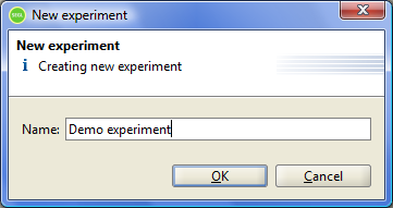
Figure 7.1: Set name of a new experiment.
After that, the program will open a new window for editing this experiment with a blank drawing area of the experiment.
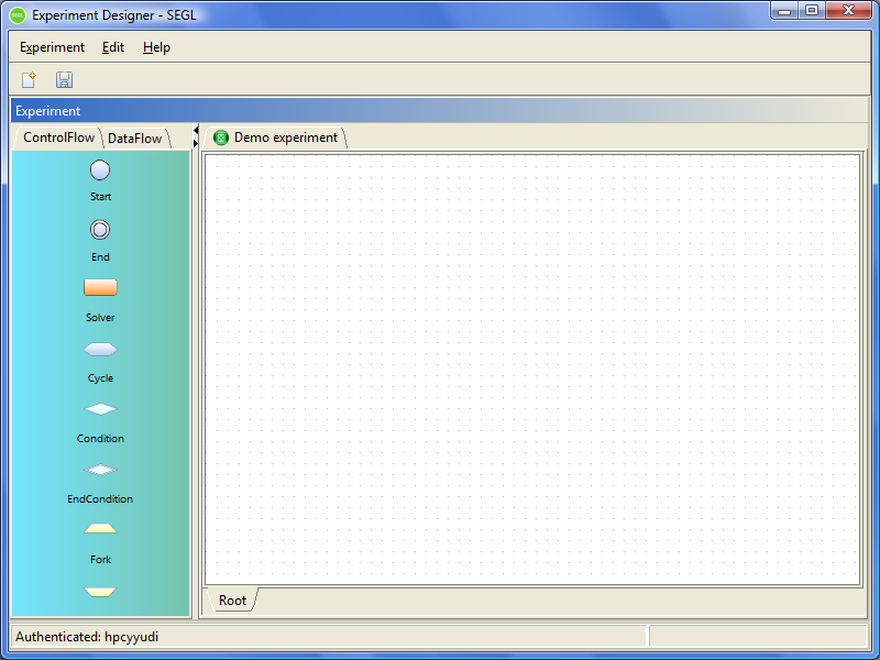
Figure 7.2: Draw area or new experiment.
The left side of the main application window contains a panel with two tabs ControlFlow and DataFlow.
These tabs contain the toolbar for editing, respectively, ControlFlow and DataFlow descriptions of the experiment. To add a new element in the drawing area, you have to drag an item from the toolbox into the drawing area.
To change the status, position or properties of an element in the drawing area, as well as to remove it, the item should be selected. Selecting an item in the drawing area is done using a single click. Selecting multiple elements is done by pressing the keys Ctrl, or by selecting a rectangular area.
Deleting selected items is done using "Delete" button on the keypad, or by choosing the context menu (right click) "Delete", or by choosing the main menu Edit→Delete.
Move the selected elements in the drawing area is performed by dragging and dropping. At the same time will be moved all selected items.
You can also change the size of any selected item.
For all items except links, you can determine the name. To do this, select an item and select the context menu, click "Properties".
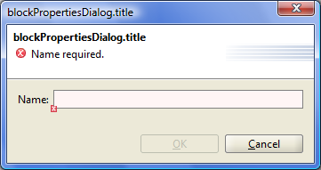
Figure 7.3: Set name of the block.
To change the name of the experiment model, move the cursor on the tab at the top of the tab bar, which shows the current name of the experiment model. Then in the context menu choose "Rename".
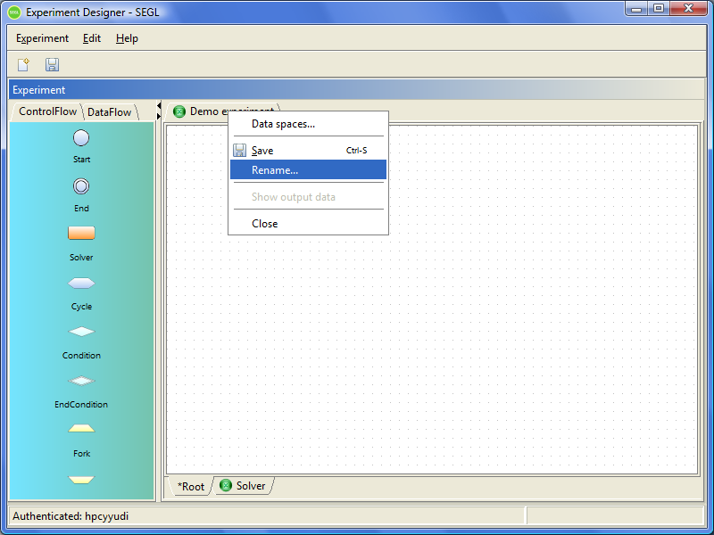
Figure 7.4: Rename experiment model.
For items such as "Solver block" and "Condition block" the user may perform editing of Data flow level.
To do this, select such block and choose "Edit" of data flow context menu. In the bottom of the tabs of this experiment will be added a new tab with the name of the selected block and the editing Data flow area of the block.
Adding links (hops) between the elements can be done in two ways:
- Connection line is added to the editing area from the toolbar. Then the ends of the line are attached (moved) to the required elements.
- Press the left mouse button on the element from which connection line should go out and move the mouse cursor on the element, in which connection line should come in and release the mouse button.
At the level of ControlFlow connecting lines may be of two types: Pipe Line and Batch line. There are two different elements in the toolbar that correspond to these types of lines. In addition, the type of lines can be changed by editing the properties of the line, using the context menu item "Properties".
IMPORTANT! On the Data flow level for such items as "Decision module" and "Computation module" connection lines are not tied to the actual modules, but to the connectors for these modules.
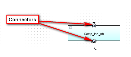
Figure 7.5: Module connectors.
Editing of Data spaces description and their usage at DataFlow is implemented as described below.
For each experiment model, there is a common set of Data spaces. To edit this set, it is necessary to to open the tab "Data spaces" from the experiment model. To do this, click on the tab with the name of the model and in the context menu, select "Data spaces".
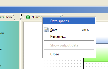
Figure 7.6: Context menu of experiment model.
After that, you will get the editing "Data spaces" tab with the object "Data spaces", which is a container for all Data spaces of the experiment model.
To add a new "Data space" in the experiment model, drag the "Data space" from the DataFlow toolbar in the container. In this case you should set properties for added Data space. The properties of the existing Data space can be changed by selecting "Properties" context menu.
In the "Name" the user should set the display name. The name must be unique within the experiment model.
In relation to the data "Data space" may be of three types: the Input data storage of the experiment, the Output data storage of the experiment and storage of the intermediate data obtained during the experiment execution.
If the Data space works with Input data of the experiment, then it must contain the default directory from which read input data for the Data space and a file name mask that defines the set of files that are will be placed in the Data space. Mask file name may contain two special values: [*] - defines any sequence of characters of any kind permitted to be in the file name, and [% i], where "i" is in the name of the actual file is an integer that specifies Dataset number for this file. These values, directory and file name may be changed for each experiment, directly before starting the experiment.
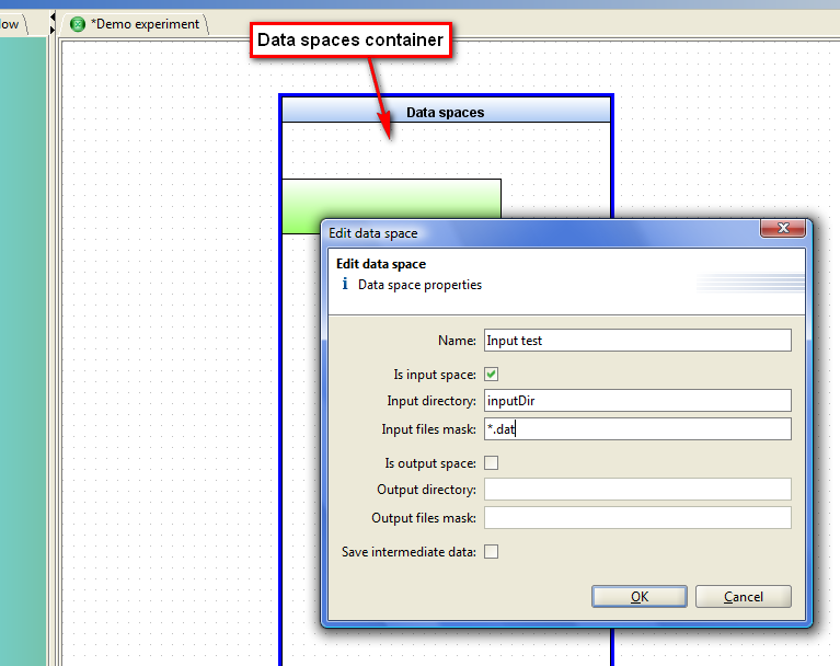
Figure 7.7: Create Data space dialog.
If the Data space keeps Output data of the experiment, the user must also set the directory name and file mask with the same special characters. Usage Data space to store output data means that if during the experiment in the Data space data will be recorded many times, in different blocks of the experiment or at different steps of the loop, then as Output data will be available the data recorded at the Data space last.
If the user finds that for the Data space after the completion of the experiment should be available all data stored in it during the experiment, it is necessary to mark the checkbox "Save intermediate data".
To describe the Data flow level of any block, you must use previously created Data spaces. To do this, in the drawing Data flow area, you have to drag "Data space" from the toolbar and put it in a Data spaces container of Data flow area. The user will be invited to select one of the Data spaces, defined in this experiment model.
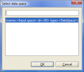
Figure 7.8: Setect Data space dialog.
Chapter 8
Start of the experiment and monitoring
To start a new experiment it is necessary to choose a model of experiment based on which a new experiment will be runned. To do this, use the main menu item Experiment→New run.
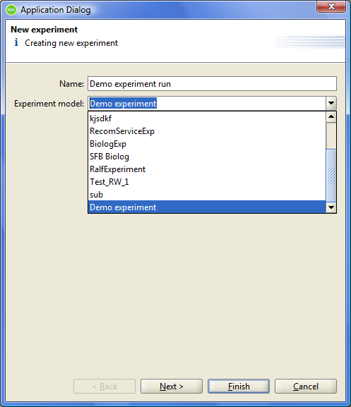
Figure 8.1: Start experiment dialog.
In the dropdown "Experiment model" the user should choose the model of the experiment, based on which an experiment will be runned. In the field "Name" the user should specify the name of the of the experiment to execute. The name of the experiment must be unique within the system. Therefore, when the user starts each new experiment based on the same model, the user must specify each time a new unique name for the experiment. If the specified name of the experiment is non-unique, the program will shown the appropriate message.
For the next step run of the experiment, click "Next". This will display the dialog for input data of the experiment.
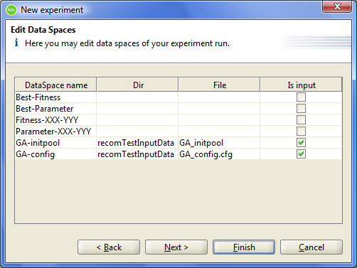
Figure 8.2: Start experiment dialog - edit Data spaces.
In this dialog all Dataspaces are displayed, as defined in the experiment model. To set the input data of the experiment such Dataspaces are used, which was defined in the model of experiment as Input dataspaces. Fields "Dir" and "File" in the table are editable fields.
In the "File" can be specified a new value for the mask or the name of the files, which will be saved in the appropriate Dataspace before starting the experiment. If this field will be given as files mask, as input in Dataspace may be referred a set of files for a set of Dataset. Also, in the file names the user can specify explicitly Datasetnumber. To do this in a mask file, the user must use the value [% i]. Then the corresponding value in the file name will be interpreted by the system as Datasetnumber. For example, if you specify a file mask "file% i.dat", then the actual files file1.dat and file2.dat will be stored in the system in the appropriate dataspace as files for Datasetnumber Datasetnumber 1 and 2, respectively.
In the file mask can also be used character *, which determines an arbitrary sequence of characters in the filename.
When editing "Dir" field, you can specify the explicitly value of directory to search input files, or call a dialog to specify the input files. To call this dialog, click on the relevant field in a table to go into edit mode of this field. And then click on the button at right side of the field.
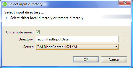
Figure 8.3: Select input directory of Data space dialog.
This dialog allows you to select as the directory to search for input Dataspace files a local directory on the computer running the client application or a remote directory on one of the HPC resources available to the user.
To specify a local directory, it is necessary that is not marked checkbox "On remote server". Than the user should select a directory in the "Directory" field.
To specify a directory on a remote resource, the user need to mark the checkbox "On remote server", select the resource in the "Server" field and set the absolute path to the directory in the "Directory" field.
IMPORTANT! The path to the remote location must be specified in absolute form. It is unacceptable to use a relative path or special symbols denoting the user's home directory. The specified directory must be accessible to the user to read files in it.
After specifying the required values for all Input dataspaces, you need to go to the next dialog to start the experiment by clicking "Next".
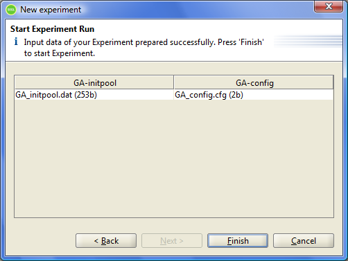
Figure 8.4: Prepared input data if experiment.
In this dialog the status of all input Dataspaces of the experiment is displayed. For each Dataspace all the found files are displayed. The user must ensure that all inputs are correctly found by the system. If the position of the input data and / or file masks were set not correctly, the user need to return to the previous step by pressing "Back".
If all inputs are defined correctly, then you can run an experiment. To do this, click "Finish". The system then begins the process of executing of the experiment. The SEGL Client application will open a new window that displays the progress of the experiment.
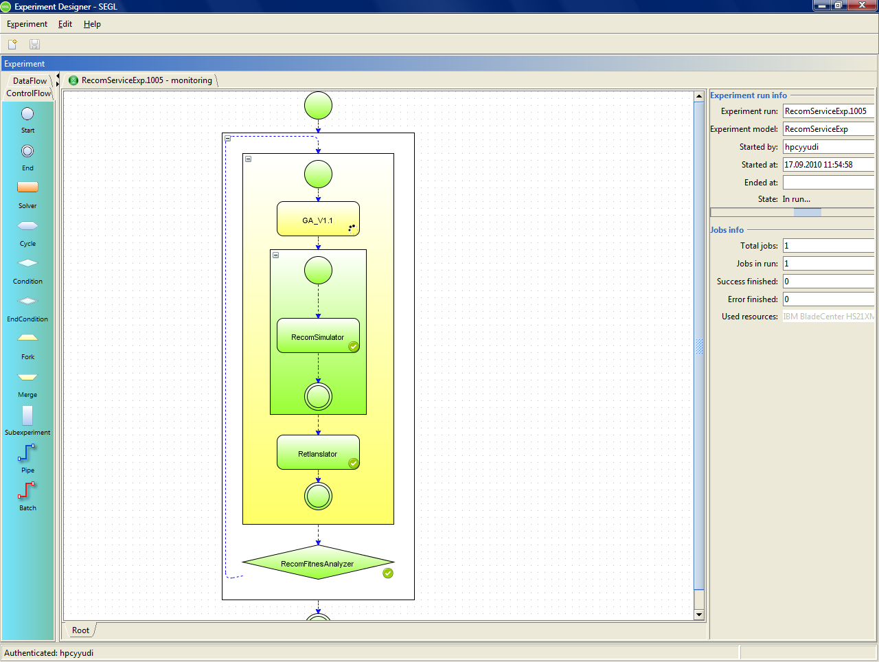
Figure 8.5: Progress of the experiment running.
From this moment, the execution of the experiment is performed on the SEGL system server, independent on the client application. Window to monitor any experiment, the currently executing or have already completed, can be opened by choosing a program menu "Experiment"→"Open experiment".
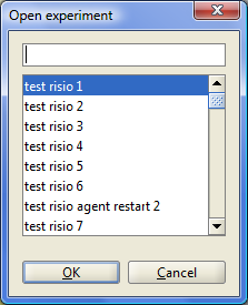
Figure 8.6: Open experiment dialog.
The monitoring window of the experiment shows Control flow description of the experiment with the animation of the currently executing block. The panel on the right side of the window displays detailed information about executing of the experiment, namely:
- number of running jobs;
- number of successfully completed jobs;
- number of jobs, which were completed with an error;
- time and date of start of the experiment;
- the name of the user running the experiment;
- current status of the experiment.
After completion of the experiment, the monitoring window will look like the figure below.
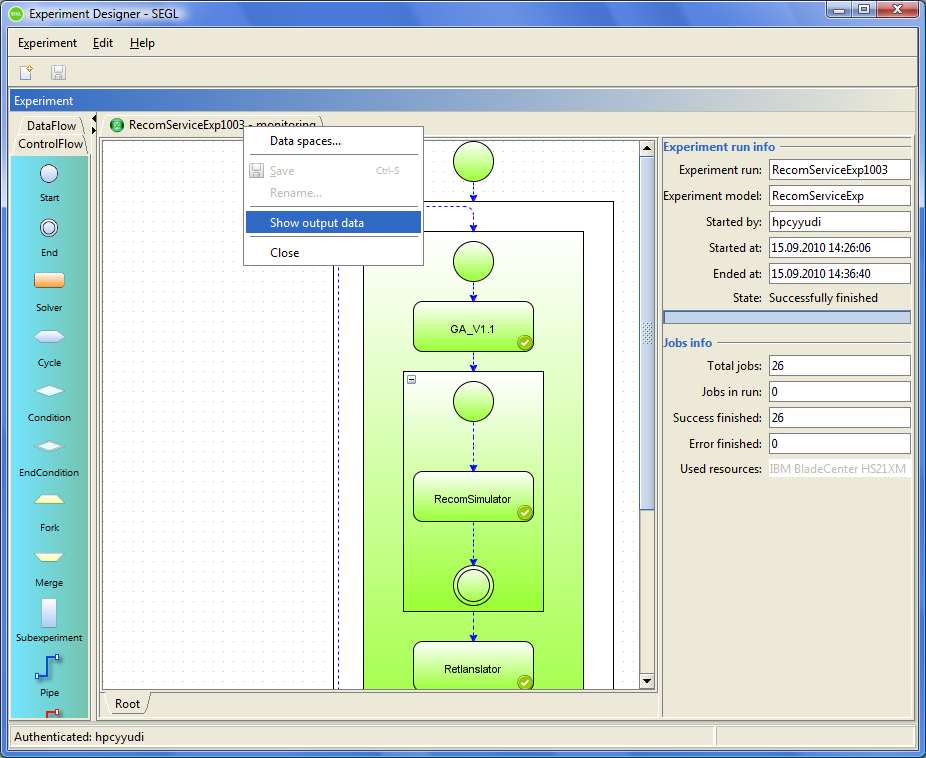
Figure 8.7: Opening a monitoring window.
After completion of the experiment, the user can get the output data of the experiment. To do this, hover over the tab with the name of the experiment and call the context menu (right-clicking on the mouse button). In the context menu the user should select the "Show ouput data" item.
After that, the system will form a tree with output data of all Dataspaces, which are marked as "Output" or "Save intermediate data" and will displays the output tree in the dialog window.
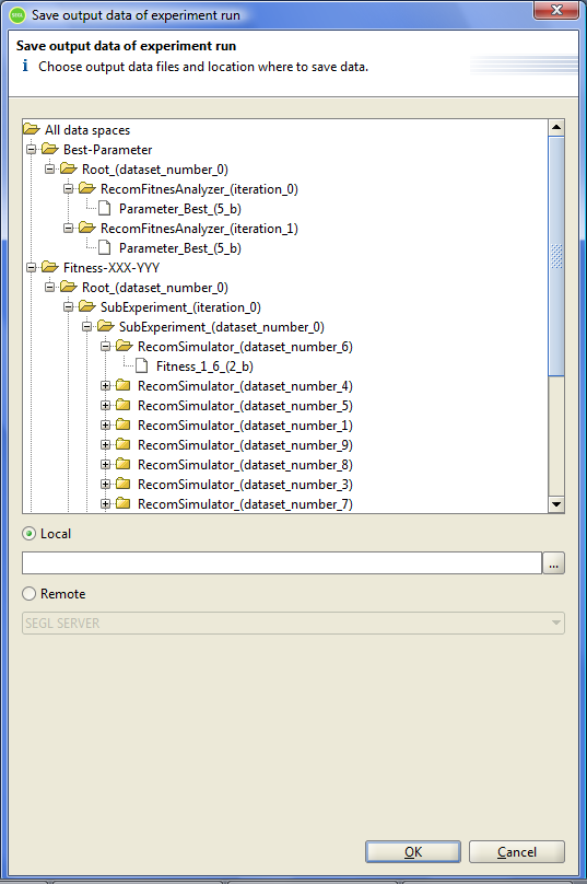
Figure 8.8: Saving output data of experiment.
This tree shows all dataspaces, marked in the model of experiment as "Output" or "Save intermediate data". Then, for each dataspace subtree of experiments is displayed in which records of output data were made in dataspace. Since in the experiment can be defined sub-experiments, in general, this will be a subtree of the experiments. Than the user can see the nodes that define the blocks, from which was stored data in the dataspace and then the actual files. Thefiles saved in different dataset, appear in different nodes of the tree.
If the block that performs data backup in the dataspace, located in a loop, all iterations of the loop will be displayed in different subtrees of the tree.
To obtain the data it is necessary to select the desired subtrees or a destination files in a tree. Such selections can be a lot and the selection is performed by pressing "Ctrl". If was selected any subtree, then all it's nodes will be saved.
After selection of the required elements in the output tree, the user must determine where to transfer the output data. This may be a user's local computer or one of the resources.
If the user selects the user's local computer (the flag "Local"), then the user must specify the folder where to save the output data of the experiment.
If the user selects a remote resource (the flag "Remote"), then the user should choose one of the resources in the dropdown list. The data will be stored in the user's home directory.
After clicking the "OK" button will start the transfer process of output user data.
It should be noted that the output data of the experiment are stored on the resource, where the tasks of the experiment were runned. In this case, the "Workspace" mechanism is used. Since the lifetime of the workspace is usually limited, the user must take care to save the data after completion of the experiment.
File translated from
TEX
by
TTH,
version 4.03.
On 24 Jan 2013, 07:54.